Análisis Factorial Confirmatorio con Indicadores Categóricos
En esta ocasión, realizaremos un análisis factorial confirmatorio con indicadores categóricos.
Iniciamos cargando los paquetes necesarios para el análisis. Los paquetes son: haven para importar datos, lavaan para estimar el análisis factorial confirmatorio (AFC), semPlot para crear gráficos de SEM y semTable para producir tablas de SEM.
# Carga paquetes
library(haven) # importar SPSS, Stata, etc.
library(summarytools)
library(dplyr)
##
## Attaching package: 'dplyr'
## The following objects are masked from 'package:stats':
##
##     filter, lag
## The following objects are masked from 'package:base':
##
##     intersect, setdiff, setequal, union
library(lavaan) # estimar SEM
## This is lavaan 0.6-16
## lavaan is FREE software! Please report any bugs.
library(semPlot) # graficar SEM
library(semTable) # tablas SEM
En este ejercicio analizaremos una escala de autoritarismo proveniente del estudio “International Civic and Citizenship Education Study 2016”.
A continuación, importamos los datos que vamos a analizar. Los datos están almacenados en un archivo .sav de SPSS llamado “ISLCHLC3.sav”. Lo importamos utilizando la función read_spss() del paquete haven.
# Importar datos
#datos <- read_spss("ISLCHLC3.sav")
datos <- read_sav(url("https://github.com/Clases-GabrielSotomayor/pruebapagina/raw/master/content/example/input/data/ISLCHLC3.sav"))
Seleccionamos y visualizamos las variables a utilizar como parte del modelo.
datos <- datos |>
  select(LS3G01A , LS3G01B, LS3G01C, LS3G01D ,
           LS3G01E , LS3G01F , LS3G02A , LS3G02B , LS3G02C)

print(dfSummary(datos, headings = FALSE, method = "render"))
##
## ---------------------------------------------------------------------------------------------------------------------------------------------------------------------
## No   Variable                               Label                                      Stats / Values          Freqs (% of Valid)   Graph         Valid     Missing
## ---- -------------------------------------- ------------------------------------------ ----------------------- -------------------- ------------- --------- ---------
## 1    LS3G01A                                Government and its leaders/It is better    Mean (sd) : 3.4 (0.8)   1 :  237 ( 4.7%)                   5049      32
##      [haven_labelled, vctrs_vctr, double]   for government leaders to make decisions   min < med < max:        2 :  405 ( 8.0%)     I             (99.4%)   (0.6%)
##                                             without consulting anybody                 1 < 4 < 4               3 : 1480 (29.3%)     IIIII
##                                                                                        IQR (CV) : 1 (0.2)      4 : 2927 (58.0%)     IIIIIIIIIII
##
## 2    LS3G01B                                Government and its leaders/People in       Mean (sd) : 3.2 (0.9)   1 :  277 ( 5.5%)     I             5037      44
##      [haven_labelled, vctrs_vctr, double]   government must enforce their authority    min < med < max:        2 :  818 (16.2%)     III           (99.1%)   (0.9%)
##                                             even if it means violating the rights      1 < 3 < 4               3 : 1512 (30.0%)     IIIIII
##                                                                                        IQR (CV) : 1 (0.3)      4 : 2430 (48.2%)     IIIIIIIII
##
## 3    LS3G01C                                Government and its leaders/People in       Mean (sd) : 2.9 (0.9)   1 :  421 ( 8.4%)     I             5020      61
##      [haven_labelled, vctrs_vctr, double]   government lose part of their authority    min < med < max:        2 : 1276 (25.4%)     IIIII         (98.8%)   (1.2%)
##                                             when they admit their mistakes             1 < 3 < 4               3 : 1930 (38.4%)     IIIIIII
##                                                                                        IQR (CV) : 2 (0.3)      4 : 1393 (27.7%)     IIIII
##
## 4    LS3G01D                                Government and its leaders/People whose    Mean (sd) : 3.3 (0.8)   1 :  229 ( 4.6%)                   5023      58
##      [haven_labelled, vctrs_vctr, double]   opinions are different than those of the   min < med < max:        2 :  482 ( 9.6%)     I             (98.9%)   (1.1%)
##                                             government must be considered its          1 < 4 < 4               3 : 1664 (33.1%)     IIIIII
##                                             enemies                                    IQR (CV) : 1 (0.2)      4 : 2648 (52.7%)     IIIIIIIIII
##
## 5    LS3G01E                                Government and its leaders/The most        Mean (sd) : 2.8 (1)     1 :  659 (13.1%)     II            5017      64
##      [haven_labelled, vctrs_vctr, double]   important opinion of a country should be   min < med < max:        2 : 1175 (23.4%)     IIII          (98.7%)   (1.3%)
##                                             that of the president                      1 < 3 < 4               3 : 1505 (30.0%)     IIIII
##                                                                                        IQR (CV) : 2 (0.4)      4 : 1678 (33.4%)     IIIIII
##
## 6    LS3G01F                                Government and its leaders/It is fair      Mean (sd) : 3.2 (0.9)   1 :  326 ( 6.5%)     I             5027      54
##      [haven_labelled, vctrs_vctr, double]   that the government does not comply with   min < med < max:        2 :  691 (13.7%)     II            (98.9%)   (1.1%)
##                                             law when it thinks it is not necessary     1 < 4 < 4               3 : 1476 (29.4%)     IIIII
##                                                                                        IQR (CV) : 1 (0.3)      4 : 2534 (50.4%)     IIIIIIIIII
##
## 7    LS3G02A                                Governments and their                      Mean (sd) : 2.7 (0.9)   1 :  537 (10.7%)     II            5028      53
##      [haven_labelled, vctrs_vctr, double]   power/Concentration of power in one        min < med < max:        2 : 1538 (30.6%)     IIIIII        (99.0%)   (1.0%)
##                                             person guarantees order                    1 < 3 < 4               3 : 1783 (35.5%)     IIIIIII
##                                                                                        IQR (CV) : 1 (0.3)      4 : 1170 (23.3%)     IIII
##
## 8    LS3G02B                                Governments and their power/The            Mean (sd) : 3.2 (0.9)   1 :  265 ( 5.3%)     I             5031      50
##      [haven_labelled, vctrs_vctr, double]   government should close communication      min < med < max:        2 :  761 (15.1%)     III           (99.0%)   (1.0%)
##                                             media that are critical                    1 < 3 < 4               3 : 1840 (36.6%)     IIIIIII
##                                                                                        IQR (CV) : 1 (0.3)      4 : 2165 (43.0%)     IIIIIIII
##
## 9    LS3G02C                                Governments and their power/If the         Mean (sd) : 2.9 (0.9)   1 :  437 ( 8.7%)     I             5006      75
##      [haven_labelled, vctrs_vctr, double]   president does not agree with              min < med < max:        2 : 1222 (24.4%)     IIII          (98.5%)   (1.5%)
##                                             <Congress>, he/she should <dissolve> it    1 < 3 < 4               3 : 1911 (38.2%)     IIIIIII
##                                                                                        IQR (CV) : 2 (0.3)      4 : 1436 (28.7%)     IIIII
## ---------------------------------------------------------------------------------------------------------------------------------------------------------------------
Definimos el modelo de medición para nuestro Análisis Factorial Confirmatorio (AFC). Estamos definiendo un factor latente (“autoritarismo”) y nueve ítems observables. El operador =~ se utiliza para indicar las relaciones entre el factor y los ítems
# Definir modelo de medicion
mod_conf <- 'autoritarismo =~ LS3G01A + LS3G01B + LS3G01C + LS3G01D +
LS3G01E + LS3G01F + LS3G02A + LS3G02B + LS3G02C'
Para ajustar el modelo utilizamos la función cfa() del paquete lavaan. Sin embargo, a diferencia de un análisis factorial confirmatorio con indicadores continuos, debemos especificar que los ítems son categóricos mediante el argumento ordered = T y el estimador utilizado es “DWLS” (Diagonally Weighted Least Squares), que es adecuado para variables categóricas.
# Ajustar modelo CFA
mod_conf_afc <- cfa(mod_conf, data = datos, estimator="DWLS", ordered = T)
Luego, visualizamos un resumen de los resultados del modelo con la función summary(). Activamos las opciones para mostrar las cargas factoriales estandarizadas (standardized = TRUE) e índices de ajuste extendidos (fit.measures = TRUE).
# Resultados
## Salida general
summary(mod_conf_afc,
        standardized = TRUE, # mostrar cargas estandarizadas
        fit.measures = TRUE) # mostrar índices de ajuste extendidos
## lavaan 0.6.16 ended normally after 19 iterations
##
##   Estimator                                       DWLS
##   Optimization method                           NLMINB
##   Number of model parameters                        36
##
##                                                   Used       Total
##   Number of observations                          4864        5081
##
## Model Test User Model:
##
##   Test statistic                               803.725
##   Degrees of freedom                                27
##   P-value (Chi-square)                           0.000
##
## Model Test Baseline Model:
##
##   Test statistic                             95756.207
##   Degrees of freedom                                36
##   P-value                                        0.000
##
## User Model versus Baseline Model:
##
##   Comparative Fit Index (CFI)                    0.992
##   Tucker-Lewis Index (TLI)                       0.989
##
## Root Mean Square Error of Approximation:
##
##   RMSEA                                          0.077
##   90 Percent confidence interval - lower         0.072
##   90 Percent confidence interval - upper         0.082
##   P-value H_0: RMSEA <= 0.050                    0.000
##   P-value H_0: RMSEA >= 0.080                    0.137
##
## Standardized Root Mean Square Residual:
##
##   SRMR                                           0.046
##
## Parameter Estimates:
##
##   Standard errors                             Standard
##   Information                                 Expected
##   Information saturated (h1) model        Unstructured
##
## Latent Variables:
##                    Estimate  Std.Err  z-value  P(>|z|)   Std.lv  Std.all
##   autoritarismo =~
##     LS3G01A           1.000                               0.792    0.792
##     LS3G01B           1.006    0.010   98.323    0.000    0.797    0.797
##     LS3G01C           0.789    0.009   87.222    0.000    0.624    0.624
##     LS3G01D           1.018    0.010  100.839    0.000    0.806    0.806
##     LS3G01E           0.900    0.009   95.097    0.000    0.713    0.713
##     LS3G01F           0.963    0.010   98.674    0.000    0.763    0.763
##     LS3G02A           0.877    0.009   93.743    0.000    0.694    0.694
##     LS3G02B           1.008    0.010  102.905    0.000    0.798    0.798
##     LS3G02C           0.882    0.009   95.410    0.000    0.698    0.698
##
## Intercepts:
##                    Estimate  Std.Err  z-value  P(>|z|)   Std.lv  Std.all
##    .LS3G01A           0.000                               0.000    0.000
##    .LS3G01B           0.000                               0.000    0.000
##    .LS3G01C           0.000                               0.000    0.000
##    .LS3G01D           0.000                               0.000    0.000
##    .LS3G01E           0.000                               0.000    0.000
##    .LS3G01F           0.000                               0.000    0.000
##    .LS3G02A           0.000                               0.000    0.000
##    .LS3G02B           0.000                               0.000    0.000
##    .LS3G02C           0.000                               0.000    0.000
##     autoritarismo     0.000                               0.000    0.000
##
## Thresholds:
##                    Estimate  Std.Err  z-value  P(>|z|)   Std.lv  Std.all
##     LS3G01A|t1       -1.684    0.031  -54.116    0.000   -1.684   -1.684
##     LS3G01A|t2       -1.140    0.023  -49.719    0.000   -1.140   -1.140
##     LS3G01A|t3       -0.203    0.018  -11.233    0.000   -0.203   -0.203
##     LS3G01B|t1       -1.608    0.030  -54.368    0.000   -1.608   -1.608
##     LS3G01B|t2       -0.783    0.020  -38.922    0.000   -0.783   -0.783
##     LS3G01B|t3        0.043    0.018    2.409    0.016    0.043    0.043
##     LS3G01C|t1       -1.386    0.026  -53.527    0.000   -1.386   -1.386
##     LS3G01C|t2       -0.422    0.019  -22.752    0.000   -0.422   -0.422
##     LS3G01C|t3        0.586    0.019   30.609    0.000    0.586    0.586
##     LS3G01D|t1       -1.702    0.031  -54.023    0.000   -1.702   -1.702
##     LS3G01D|t2       -1.076    0.022  -48.210    0.000   -1.076   -1.076
##     LS3G01D|t3       -0.072    0.018   -3.985    0.000   -0.072   -0.072
##     LS3G01E|t1       -1.125    0.023  -49.373    0.000   -1.125   -1.125
##     LS3G01E|t2       -0.346    0.018  -18.829    0.000   -0.346   -0.346
##     LS3G01E|t3        0.421    0.019   22.695    0.000    0.421    0.421
##     LS3G01F|t1       -1.524    0.028  -54.332    0.000   -1.524   -1.524
##     LS3G01F|t2       -0.838    0.020  -40.941    0.000   -0.838   -0.838
##     LS3G01F|t3       -0.013    0.018   -0.717    0.473   -0.013   -0.013
##     LS3G02A|t1       -1.253    0.024  -51.848    0.000   -1.253   -1.253
##     LS3G02A|t2       -0.223    0.018  -12.320    0.000   -0.223   -0.223
##     LS3G02A|t3        0.724    0.020   36.571    0.000    0.724    0.724
##     LS3G02B|t1       -1.624    0.030  -54.339    0.000   -1.624   -1.624
##     LS3G02B|t2       -0.829    0.020  -40.625    0.000   -0.829   -0.829
##     LS3G02B|t3        0.175    0.018    9.687    0.000    0.175    0.175
##     LS3G02C|t1       -1.357    0.025  -53.236    0.000   -1.357   -1.357
##     LS3G02C|t2       -0.435    0.019  -23.376    0.000   -0.435   -0.435
##     LS3G02C|t3        0.563    0.019   29.547    0.000    0.563    0.563
##
## Variances:
##                    Estimate  Std.Err  z-value  P(>|z|)   Std.lv  Std.all
##    .LS3G01A           0.373                               0.373    0.373
##    .LS3G01B           0.365                               0.365    0.365
##    .LS3G01C           0.610                               0.610    0.610
##    .LS3G01D           0.351                               0.351    0.351
##    .LS3G01E           0.492                               0.492    0.492
##    .LS3G01F           0.418                               0.418    0.418
##    .LS3G02A           0.518                               0.518    0.518
##    .LS3G02B           0.364                               0.364    0.364
##    .LS3G02C           0.512                               0.512    0.512
##     autoritarismo     0.627    0.009   73.038    0.000    1.000    1.000
##
## Scales y*:
##                    Estimate  Std.Err  z-value  P(>|z|)   Std.lv  Std.all
##     LS3G01A           1.000                               1.000    1.000
##     LS3G01B           1.000                               1.000    1.000
##     LS3G01C           1.000                               1.000    1.000
##     LS3G01D           1.000                               1.000    1.000
##     LS3G01E           1.000                               1.000    1.000
##     LS3G01F           1.000                               1.000    1.000
##     LS3G02A           1.000                               1.000    1.000
##     LS3G02B           1.000                               1.000    1.000
##     LS3G02C           1.000                               1.000    1.000
Además, podemos ver solo los índices de ajuste específicos que nos interesan utilizando la función fitmeasures().
# Ver solo indices de ajuste
fitmeasures(mod_conf_afc,
            fit.measures = c("chisq", "df", "pvalue",
                             "cfi", "rmsea"))
##   chisq      df  pvalue     cfi   rmsea
## 803.725  27.000   0.000   0.992   0.077
Los índices de ajuste incluyen la chi-cuadrada (chisq), los grados de libertad (df), el p-valor (pvalue), el índice de ajuste comparativo (cfi), y el error cuadrático medio de aproximación (rmsea). Estos índices nos ayudan a evaluar qué tan bien se ajusta el modelo a nuestros datos.
A continuación, creamos un gráfico del modelo usando la función semPaths(). La opción what = “std” se utiliza para mostrar las cargas factoriales estandarizadas en el gráfico.
# Diagrama modelo
semPaths(mod_conf_afc, # modelo ajustado
         what = "std",  # mostrar cargas estandarizadas
         label.cex = 1, edge.label.cex = 1, # tamaño flechas y caracteres
         residuals = FALSE, # no mostrar residuos
         edge.color = "black") # color flechas
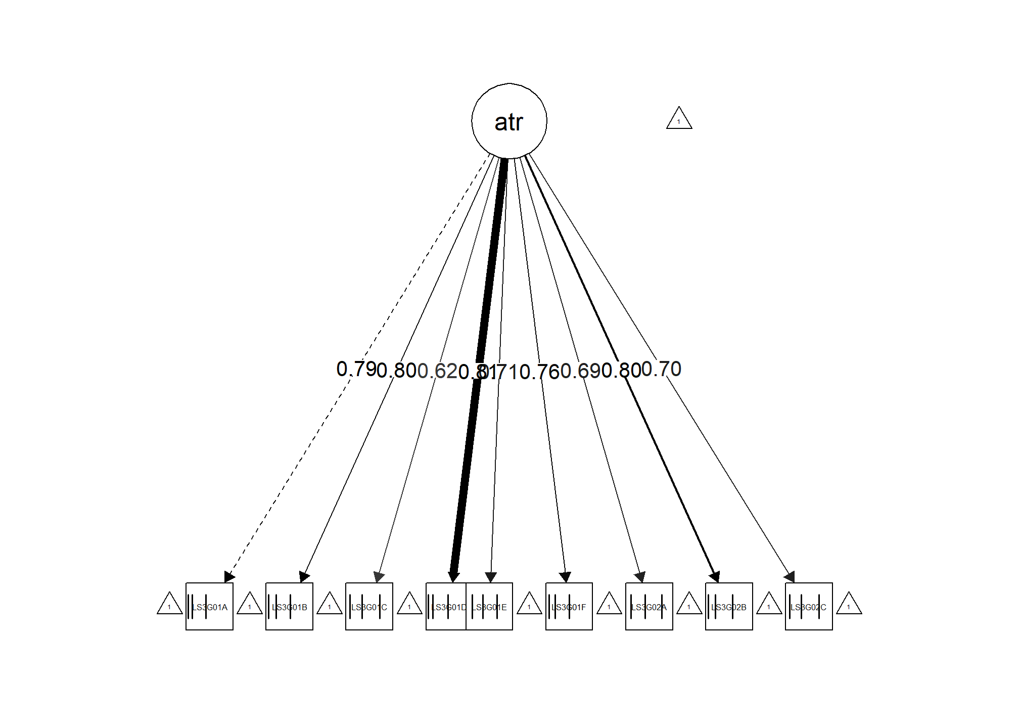 Para interpretar el gráfico, las flechas representan las relaciones entre el factor latente y los ítems. Los números en las flechas son las cargas factoriales estandarizadas, que indican la fuerza de la relación entre cada ítem y el factor.
A continuación, calculamos las comunalidades, que son las proporciones de varianza de cada ítem que se explican por el factor. Usamos la función inspect() con what = “rsquare” para hacer esto.
# Comunalidades
inspect(mod_conf_afc, what = "rsquare")
## LS3G01A LS3G01B LS3G01C LS3G01D LS3G01E LS3G01F LS3G02A LS3G02B LS3G02C
##   0.627   0.635   0.390   0.649   0.508   0.582   0.482   0.636   0.488
Por último, revisamos los índices de modificación, que sugieren cambios potenciales al modelo que podrían mejorar el ajuste. Mostramos los índices en orden decreciente para identificar los cambios más impactantes primero.
# Indices de modificacion
## Mostrar 'mi' en orden decreciente
modificationindices(mod_conf_afc, sort. = T)
##         lhs op     rhs      mi    epc sepc.lv sepc.all sepc.nox
## 101 LS3G02B ~~ LS3G02C 184.051  0.148   0.148    0.343    0.343
## 100 LS3G02A ~~ LS3G02C 120.146  0.125   0.125    0.243    0.243
## 66  LS3G01A ~~ LS3G01B 112.821  0.119   0.119    0.321    0.321
## 99  LS3G02A ~~ LS3G02B 104.847  0.118   0.118    0.272    0.272
## 89  LS3G01D ~~ LS3G02A  61.539 -0.112  -0.112   -0.263   -0.263
## 73  LS3G01A ~~ LS3G02C  58.349 -0.112  -0.112   -0.257   -0.257
## 80  LS3G01B ~~ LS3G02C  56.790 -0.103  -0.103   -0.239   -0.239
## 79  LS3G01B ~~ LS3G02B  46.309 -0.085  -0.085   -0.234   -0.234
## 84  LS3G01C ~~ LS3G02A  37.485 -0.082  -0.082   -0.147   -0.147
## 98  LS3G01F ~~ LS3G02C  34.085 -0.080  -0.080   -0.173   -0.173
## 91  LS3G01D ~~ LS3G02C  32.975 -0.078  -0.078   -0.184   -0.184
## 88  LS3G01D ~~ LS3G01F  31.579  0.065   0.065    0.170    0.170
## 85  LS3G01C ~~ LS3G02B  24.764 -0.067  -0.067   -0.142   -0.142
## 71  LS3G01A ~~ LS3G02A  24.697 -0.073  -0.073   -0.165   -0.165
## 96  LS3G01F ~~ LS3G02A  24.319 -0.069  -0.069   -0.148   -0.148
## 72  LS3G01A ~~ LS3G02B  21.959 -0.060  -0.060   -0.162   -0.162
## 78  LS3G01B ~~ LS3G02A  19.403 -0.059  -0.059   -0.136   -0.136
## 82  LS3G01C ~~ LS3G01E  16.903  0.052   0.052    0.094    0.094
## 81  LS3G01C ~~ LS3G01D  16.692  0.052   0.052    0.113    0.113
## 94  LS3G01E ~~ LS3G02B  11.794 -0.044  -0.044   -0.103   -0.103
## 86  LS3G01C ~~ LS3G02C  11.782 -0.045  -0.045   -0.081   -0.081
## 68  LS3G01A ~~ LS3G01D  10.762  0.039   0.039    0.108    0.108
## 83  LS3G01C ~~ LS3G01F   8.812  0.039   0.039    0.078    0.078
## 97  LS3G01F ~~ LS3G02B   7.148 -0.033  -0.033   -0.085   -0.085
## 74  LS3G01B ~~ LS3G01C   6.864  0.034   0.034    0.071    0.071
## 93  LS3G01E ~~ LS3G02A   6.805  0.033   0.033    0.065    0.065
## 90  LS3G01D ~~ LS3G02B   6.575 -0.030  -0.030   -0.085   -0.085
## 69  LS3G01A ~~ LS3G01E   5.668 -0.033  -0.033   -0.077   -0.077
## 75  LS3G01B ~~ LS3G01D   2.363  0.018   0.018    0.050    0.050
## 77  LS3G01B ~~ LS3G01F   1.290  0.014   0.014    0.035    0.035
## 70  LS3G01A ~~ LS3G01F   0.972  0.012   0.012    0.031    0.031
## 92  LS3G01E ~~ LS3G01F   0.734  0.011   0.011    0.024    0.024
## 87  LS3G01D ~~ LS3G01E   0.597 -0.010  -0.010   -0.024   -0.024
## 67  LS3G01A ~~ LS3G01C   0.349 -0.008  -0.008   -0.018   -0.018
## 95  LS3G01E ~~ LS3G02C   0.092  0.004   0.004    0.008    0.008
## 76  LS3G01B ~~ LS3G01E   0.070 -0.003  -0.003   -0.008   -0.008
Estos índices pueden ayudarte a mejorar tu modelo. Sin embargo, cualquier cambio que hagas en el modelo basándote en estos índices debe tener sentido teórico. No es recomendable hacer cambios al modelo solo porque los índices de modificación sugieran que mejorarán el ajuste.